Chapter 2 R basics

2.1 Overview

This chapter covers some basic tools and characteristics of the R language that we’ll use in the workshop. While this obviously can’t be a comprehensive introduction to R, we’ll demonstrate some essential R notions and features that are commonly used in social science data analysis, including (egocentric) social network analysis.

The script covers the following topics:

• Starting R, getting help with R.
• Creating and saving R objects.
• Vectors and matrices, data frames and tibbles.
• Arithmetic and relational operations.
• Subsetting vectors, matrices, and data frames.

2.2 Starting R and loading packages

• Before starting any work in R, you normally want to do two things:
  • Make sure your R session is pointing to the correct working directory.
  • Install and/or load the packages you are going to use.
• Working directory. By default, R will look for files and save new files in this directory.
  • Type getwd() in the console to view your current working directory.
  • If you opened RStudio by double-clicking on a project (.Rproj) file, then the working directory is the folder where that file is located.
  • You can always use setwd() to manually change your working directory to any path, but it’s usually more convenient to work with R projects and their default working directory instead.
  • In RStudio, you can also check the current working directory by clicking on the Files panel.
• R packages. There are two steps to using a package in R:
  1. Install the package. You do this just once. Use install.packages("package_name") or the appropriate RStudio menu (Tools > Install Packages...). Once you install a package, the package files are in your system R folder and R will be able to always find the package there.
  2. Load the package in your current session. Use library(package_name) (no quotation marks around the package name). You do this in each R session in which you need the package, that is, every time you start R and you need the package.
• An R package is just a collection of functions. You can only use an R function if that function is included in a package you loaded in the current session.
• Sometimes two different functions from two different packages have the same name. For example, both the igraph package and the sna package have a function called degree. If both packages are loaded, typing just degree might give you unexpected results, because R will pick one of the two functions (the one in the package that was loaded most recently), which might not be the function you meant.
  • To avoid this problem, you can use the package::function() notation: igraph::degree() will always call the degree function from the igraph package, while sna::degree() will call the degree function from the sna package.
• Tip: To check the package that a function comes from, just go to that function’s manual page. The package will be indicated in the first line of the page. E.g., type ?degree to see where the degree function comes from.
  • If no currently loaded package has a function called degree, then typing ?degree will cause a warning (No documentation for 'degree').
  • If multiple, currently loaded packages have a function called degree, then typing ?degree will bring up a page with the list of all those packages.
• This workshop will use a number of packages, listed here.

2.2.1 Console vs scripts

• When you open RStudio, you typically see two separate windows: the script editor and the console. You can write R code in either of them.
• Console. Here you write R code line by line. Once you type a line, you press ENTER to execute it. By pressing ARROW UP you go back to the last line you ran. By continuing to press ARROW UP, you can navigate through all the lines of code you previously executed. This is called the “commands history” (all the lines of code executed in the current session). You will lose all this code (all the history) when you quit R, unless you explicitly save the history to a file (which is not what you typically do, you should just write the code in a script).
  
• Script editor. Here you write a script. This is the most common way of working with R. A script is simply a plain text file where all your R code is saved. If your work is in a script, it is reproducible.
• Both the R standard GUI and RStudio have a script editor with several helpful tools. Among other things, these allow you to run a script while you write it. By pressing CTRL+ENTER (Windows) or CMD+ENTER (Mac), you run the script line your cursor is on (or the selected script region).
  • Note that with RStudio you can run the single script line where your cursor is; a whole highlighted region of code; the region of code from the beginning of the script up to the line where your cursor is; the region of code from the line where your cursor is up to the end of the script. See the Code menu and its keyboard shortcuts.
• The script editor also allows you to save your script. In RStudio, see File > Save and its keyboard shortcut. R script files commonly have a .R extension (e.g. “myscript.R”). But note that a script file is just a text file (like any .txt file), which you can open and edit in any text editor, or in Microsoft Word and the likes.
• You can also run a whole script altogether — this is called sourcing a script. By running source("myscript.R"), you source the script file myscript.R (assuming the file is in your working directory, otherwise you’ll have to enter the whole file path). In RStudio: see Code > Source and its keyboard shortcut.
• In both the console and the script editor, any line that starts by # is called a comment. R disregards comments — it just prints them as they are in the console (does not parse and execute them as programming code). Remember to always use comments to document what your code is doing (this is good for yourself and for others).
• In RStudio you can navigate the script headings in your script with a drop-down menu in the bottom-left of the script editor. Any line that starts by # and ends by ####, ----, or ==== is read as a heading by RStudio.

2.2.2 Getting help

• Getting help is one of the most common things you do when using R. As a beginner, you’ll constantly need to get help (for example, read manual pages) about R functions. Also as an experienced user, you’ll often need to go back to the manual pages of particular functions or other R help resources. At any experience level, using R involves constantly using its documentation and help resources.
• The following are a few help tools in R:
  • help(...) or ?... are the most common ways of getting help: they send you to the R manual page for a specific function. E.g. help(sum) or ?sum (they are equivalent).
  • help.start() (or RStudio: Help > R Help) gives you general help pages in html (introduction to R, references to all functions in all installed packages, etc.).
  • demo() gives you demos on specific topics. Run demo() to see all available topics.
  • example() gives you example code on specific functions, e.g. example(sum) for the function sum.
    
  • help.search(...) or ??... search for a specific string in the manual pages, e.g. ??histogram.
• In addition to built-in help facilities within R, there are plenty of ways to get R help online. Certain popular R packages have their own website, e.g. ggplot2, igraph, and statnet. Other websites for general R help include rdocumentation.org and stackoverflow.com. See the workshop slides or talk to me for more information.

# What's the current working directory? 
# getwd() 
# Un-comment to check your actual working directory.

# Change the working directory. 
# setwd("/my/working/directory") 
# (Delete the leading "#" and type in your actual working directory's path
# instead of "/my/working/directory")

# You should use R projects (.Rproj) to point to a working directory instead of
# manually changing it.

# Suppose that we want to use the package "igraph" in the following code.
library(igraph)

# Note that we can only load a package if we have it installed. In this case, I
# have igraph already installed. Had this not been the case, I would have have
# needed to install it: 
# install.packages("igraph").
# (Packages can also be installed through an RStudio menu item).

# Let's load another suite of packages we'll use in the rest of this script.
library(tidyverse)

# Note that whatever is typed after the "#" sign has no effect but to be printed
# as is in the console: it is a comment.

2.3 Objects in R

In R, everything that exists is an object. Everything that happens is a function call. - John Chambers

• R is an object-oriented programming language. Everything is contained in an object, including data, analysis tools and analysis results. Things such as datasets, commands (called “functions” in R), regression results, descriptive statistics, etc., are all objects.
• An object has a name and a value. You create an object by assigning a value to a name.
  • You assign with <- or with =.
  • R is case-sensitive: the object named mydata is different from the object named Mydata.
• Whenever you run an operation or execute a function in R, you need to assign the result to an object if you want to save it and re-use it later. Assign it or lose it: anything that is not assigned to an object is just printed to the console and lost.
• Objects have a size (bytes, megabytes, etc.) and a type (technically, a class, a type and a mode — more on this later).
• A function is a particular type of object. Functions take other objects as arguments (input) and return more objects as a result (output). R functions are what other data analysis programs call “commands”. See Section 8.1.2 for more about functions.

2.3.1 The workspace

• During your R session, objects (data, results) are located in the computer’s main memory. They make up your workspace: the set of all the objects currently in memory. They will disappear when you quit R, unless you save them to files on disk.
• What’s in your current workspace?
  • The function ls() shows you a full list of the objects currently in the workspace.
  • Alternatively, in RStudio open the Environment panel to get a clickable list of objects currently in the workspace (if you don’t see your Environment panel, check Preferences... > Pane Layout).

2.3.2 Saving and removing objects

• Two main functions to save R objects to files: save() (saves specific objects, its arguments); save.image() (saves all the current workspace).
• Unless you specify a different path, all files you save from R are put in your current working directory.
• The most common file extensions for files that store R objects are .rda and .RData.
• If you have a file with R objects, say objects.rda, you can load it in you current R session using the load() function: load(file= "objects.rda"). This assumes objects.rda is in your current working directory (otherwise you’ll have to specify the whole file path).
• The function rm() removes specific objects from the workspace. You can use it to clear the workspace from all existing objects by typing rm(list=ls()) (remember that ls() returns a character vector with the names of all the objects in the current workspace).

# Create the object a: assign the value 50 to the name "a"
a <- 50

# Display ("print") the object a.
a

## [1] 50

# Let's create another object.
b <- "Mark"

# Display it.
b

## [1] "Mark"

# Create and display object at the same time.
(obj <- 10)

## [1] 10

# Let's reuse the object we created for a simple operation.
a + 3

## [1] 53

# What if we want to save this result?
result <- a + 3

# All objects in the workspace
ls()

## [1] "a"      "b"      "obj"    "result"

# Now we can view that result whenever we need it.
result

## [1] 53

# ...and further re-use it
result*2

## [1] 106

# Note that R is case-sensitive, "result" is different from "reSult".
reSult

## Error in eval(expr, envir, enclos): object 'reSult' not found

# Let's clear the workspace before proceeding.
rm(list=ls())

# The workspace is now empty.
ls()

## character(0)

2.3.3 Vector and matrix objects

• Vectors are the most basic objects you use in R. Vectors can be numeric (numerical data), logical (TRUE/FALSE data), or character (string data).
• The basic function to create a vector is c (concatenate).
• Other useful functions to create vectors: rep and seq.
  • Another function we’ll use to create vectors later in the workshop is seq_along. seq_along(x) creates a vector consisting of a sequence of integers from 1 to length(x) in steps of 1.
  • Also keep in mind the : shortcut: c(1, 2, 3, 4) is the same as 1:4.
• The length (number of elements) is a basic property of vectors: length(x) returns the length of vector x.
• When we print vectors, the numbers in square brackets indicate the positions of vector elements.
• To create a matrix: matrix. Its main arguments are the cell values (within c()), number of rows (nrow) and number of columns (ncol). Values are arranged in a nrow x ncol matrix by column. See ?matrix.
• When we print matrices, the numbers in square brackets indicate the row and column numbers.

2.3.4 Data frames

• “Data frame” is R’s name for dataset. A dataset is a collection of cases (rows), and variables (columns) which are measured on those cases.
• When printed in R, data frames look like matrices. However, unlike matrix columns, data frame columns can be of different types, e.g. a numeric variable and a character variable.
• On the other hand, just like matrix columns, data frame columns (variables) must all have the same length (number of cases). You can’t put together variables (vectors) of different length in the same data frame.
• Although data frames look like matrices, in R’s mind they are a specific kind of list (more about lists in Section 5.3). In fact, the class of a data frame is data.frame, but the type of a data frame is list. The list elements for a data frame are its variables (columns).
• Tibbles. The tidyverse packages, which we use in this workshop, rely on a more efficient form of data frame, called tibble.
  • A tibble has class tbl_df and data.frame. This means that, to R, a tibble is also a data frame, and any function that works on data frames normally also works on tibbles.
  • A tibble has a number of advantages over a traditional data frame, some of which we’ll see in this workshop.
  • One of the advantages is the clearer and more informative way in which tibbles are printed. When we print a tibble data frame we can immediately see its number of rows, number of columns, names of variables, and type of each variable (numeric, integer, character, etc.).
  • To convert an existing data frame to tibble: as_tibble. To create a tibble from scratch (similar to the data.frame function in base R): tibble.
• While data frames can be created manually in R (with the functions data.frame in base R and tibble in tidyverse), data are most commonly imported into R from external sources, like a csv or txt file.
• We’ll import data from csv files using the read_csv() function from tidyverse.
  • read_csv() reads csv files (values separated by “,” or “;”). read_delim() reads files in which values are separated by any delimiter.
  • These functions have many arguments that make them very flexible and allow users to import basically any kind of table stored in a text file. Check out ?read_delim.
  • In base R, the corresponding functions are read.csv() and read.table().
• Data can also be imported into R from most external file formats (SAS, SPSS, Stata, Excel, etc.) using the tidyverse packages readxl and haven, or the foreign package in traditional R.
• Note that you can click on a data frame’s name in RStudio’s Environment pane. That will open the data frame in a window, similar to SPSS’s data view.

# Let's create a simple vector.
(x <- c(1, 2, 3, 4))

## [1] 1 2 3 4

# Shortcut for the same thing.
(y <- 1:4)

## [1] 1 2 3 4

# What's the length of x?
length(x)

## [1] 4

# Note that when we print vectors, numbers in square brackets indicate positions
# of the vector elements.

# Create a simple matrix.
adj <- matrix(c(0,1,0, 1,0,0, 1,1,0), nrow= 3, ncol=3)

# This is what our matrix looks like:
adj

##      [,1] [,2] [,3]
## [1,]    0    1    1
## [2,]    1    0    1
## [3,]    0    0    0

# Notice the row and column numbers in square brackets. 

# Normally we create data frames by importing data from external files, for
# example csv files.
ego.df <- read_csv("./Data/raw_data/ego_data.csv")

## Rows: 102 Columns: 9
## ── Column specification ────────────────────────────────────────────────────────
## Delimiter: ","
## chr (4): ego.sex, ego.edu, ego.empl.bin, ego.age.cat
## dbl (5): ego_ID, ego.age, ego.arr, ego.inc, empl
## 
## ℹ Use `spec()` to retrieve the full column specification for this data.
## ℹ Specify the column types or set `show_col_types = FALSE` to quiet this message.

# View the result.
ego.df

## # A tibble: 102 × 9
##    ego_ID ego.sex ego.age ego.arr ego.edu ego.inc  empl ego.empl.bin ego.age.cat
##     <dbl> <chr>     <dbl>   <dbl> <chr>     <dbl> <dbl> <chr>        <chr>      
##  1     28 Male         61    2008 Second…     350     3 Yes          60+        
##  2     29 Male         38    2000 Primary     900     4 Yes          36-40      
##  3     33 Male         30    2010 Primary     200     3 Yes          26-30      
##  4     35 Male         25    2009 Second…    1000     3 Yes          18-25      
##  5     39 Male         29    2007 Primary       0     1 No           26-30      
##  6     40 Male         56    2008 Second…     950     4 Yes          51-60      
##  7     45 Male         52    1975 Primary    1600     3 Yes          51-60      
##  8     46 Male         35    2002 Second…    1200     4 Yes          31-35      
##  9     47 Male         22    2010 Second…     700     4 Yes          18-25      
## 10     48 Male         51    2007 Primary     950     4 Yes          51-60      
## # ℹ 92 more rows

# Note the different pieces of information that are displayed when printing a tibble
# data frame.

2.4 Arithmetic, statistical, and relational operations

2.4.1 Arithmetic operations and recycling

• R can work as a normal calculator.
  • Addition/subtraction: 7+3
  • Multiplication: 7*3
  • Negative: -7
  • Division: 7/3
  • Integer division: 7%/%3
  • Integer remainder: 7%%3
  • Exponentiation: 7^3
• Many operations involving vectors in R are performed element-wise, i.e., separately on each element of the vector (see examples below).
• Most operations on vectors use the recycling rule: if a vector is too short, its values are re-used the number of times needed to match the desired length (see examples below).
• Examples of vector operations and recycling:
  • [1 2 3 4] + [1 2 3 4] = [1+1 2+2 3+3 4+4] (element-wise addition.)
  • [1 2 3 4] + 1 = [1+1 2+1 3+1 4+1] (1 is recycled 3 times to match the length of the first vector.)
  • [1 2 3 4] + [1 2] = [1+1 2+2 3+1 4+2] ([1 2] is recycled once.)
  • [1 2 3 4] + [1 2 3] = [1+1 2+2 3+3 4+1] ([1 2 3] is recycled one third of a time: R will warn that the length of longer vector is not a multiple of the length of shorter vector.)

2.4.2 Relational operations and logical vectors

• Relational operators: >, <, <=, >=. Equal is == (NOT =). Not equal is !=.
  • Note: equal is ==, whereas = has a different meaning. = is used to assign function arguments (e.g. matrix(x, nrow = 3, ncol = 4)), or to assign objects (x <- 2 is the same as x = 2).
• Relational operations result in logical vectors: vectors of TRUE/FALSE values.
• Like arithmetic operations, relational ones are performed element-wise on vectors, and recycling applies.
• Logical operators: & for AND, | for OR.
• Negation (i.e. opposite) of a logical vector: !.
• Is value x in vector y? x %in% y.
• R can convert logical vectors to numeric (as.numeric(), as.integer()). In this conversion, TRUE becomes 1 and FALSE becomes 0. Conversely, if converted to logical (as.logical()), 1/0 are TRUE/FALSE.
  • Therefore, if x is a logical vector, sum(x) gives the count of TRUEs in x (sum of 1s in the vector).
  • mean(x) gives the proportion of 1s in x (mean of a binary vector: sum of 1s in the vector divided by number of elements in the vector).

2.4.3 Examples of arithmetic and statistical functions

• Arithmetic vector functions are performed element-wise, and return a vector. Examples:
  • Exponential: exp(x).
  • Logarithm: log(x) (base e) or log10(x) (base 10).
• Statistical scalar functions are executed on the set of all vector elements taken together, and return a scalar. Examples:
  • mean(x) and median(x).
  • Standard deviation and variance: sd(x), var(x).
  • Minimum and maximum: min(x), max(x).
  • sum(x): sum of all elements in x.
• table(x) is another basic statistical function (but it’s not scalar):
  • table(x) returns a table object with the absolute frequencies of values in x.
• Functions such as sum(), mean() and table() are very useful when programming in R (for example, when writing your own functions). However, if you just need descriptive statistics for the data, there are more convenient tools you can use. Some of these are the following functions, which work well with tidyverse (we’ll see them in Ch. 4):
  • The skim function (from the skimr package) for descriptive statistics of continuous/quantitative variables.
  • The tabyl function (from the janitor package) for frequencies of categorical variables.

2.4.4 Missing and infinite values

• Missing values in R are represented by NA (Not Available).
  • If your data has a different code for missing values (e.g., -99), you’ll have to recode that to NA for R to properly handle missing values in your data.
• Infinity may result from arithmetic operations: Inf and -Inf (e.g. 3/0). NaN also may result, meaning Not a Number (e.g. 0/0).
  • While NAs can appear in any type of object, Inf, -Inf and NaN can only appear in numeric objects.
• is.na(x) checks if each element of x is NA and returns TRUE if that’s the case, FALSE otherwise. It’s a vector function (its value has the same length as x).

# Just a few arithmetic operations between vectors to demonstrate element-wise
# calculations and the recycling rule.

(v1 <- 1:4)

## [1] 1 2 3 4

(v2 <- 1:4)

## [1] 1 2 3 4

# [1 2 3 4] + [1 2 3 4]
v1 + v2

## [1] 2 4 6 8

# [1 2 3 4] + 1
1:4 + 1

## [1] 2 3 4 5

# [1 2 3 4] + [1 2]
(v1 <- 1:4)

## [1] 1 2 3 4

(v2 <- 1:2)

## [1] 1 2

v1 + v2

## [1] 2 4 4 6

# [1 2 3 4] + [1 2 3]
1:4 + 1:3

## Warning in 1:4 + 1:3: longer object length is not a multiple of shorter object
## length

## [1] 2 4 6 5

# Relational operations.

# Let's take a single variable from the ego attribute data: ego's age (in years)
# for the first 10 respondents. Let's put the result in a separate vector. This
# code involves indexing, we'll explain it better below.
age <- ego.df$ego.age[1:10]
age

##  [1] 61 38 30 25 29 56 52 35 22 51

# Note how the following comparisons are performed element-wise, and the value
# to which age is compared (30) is recycled.

# Is age equal to 30?
age==30

##  [1] FALSE FALSE  TRUE FALSE FALSE FALSE FALSE FALSE FALSE FALSE

# The resulting logical vector is TRUE for those elements (i.e., respondents)
# who meet the condition.

# Which respondent's age is greater than 40?
age > 40

##  [1]  TRUE FALSE FALSE FALSE FALSE  TRUE  TRUE FALSE FALSE  TRUE

# Which respondent age values are lower than 40 OR greater than 60?
age < 40 | age > 60

##  [1]  TRUE  TRUE  TRUE  TRUE  TRUE FALSE FALSE  TRUE  TRUE FALSE

# Which elements of "age" are lower than 40 AND greater than 30?
age < 40 & age > 30

##  [1] FALSE  TRUE FALSE FALSE FALSE FALSE FALSE  TRUE FALSE FALSE

# Notice the difference between OR (|) and AND (&).

# Is 30 in "age"? I.e., is one of the respondents of 30 years of age?
30 %in% age

## [1] TRUE

# Is "age" in c(30, 35)? That is, which values of "age" are either 30 or 35?
age %in% c(30, 35)

##  [1] FALSE FALSE  TRUE FALSE FALSE FALSE FALSE  TRUE FALSE FALSE

# A logical vector can be converted to numeric: TRUE becomes 1 and FALSE becomes
# 0.
age > 45

##  [1]  TRUE FALSE FALSE FALSE FALSE  TRUE  TRUE FALSE FALSE  TRUE

as.numeric(age > 45)

##  [1] 1 0 0 0 0 1 1 0 0 1

# This allows us to use the sum() and the mean() functions to get the count and
# proportion of TRUE's in a logical vector.

# Count of TRUE's: Number of respondents (elements of "age") that are older than
# 40.
sum(age > 45)

## [1] 4

# How many respondents in the vector are older than 30?
sum(age > 30)

## [1] 6

# Proportion of TRUE's: What's the proportion of "age" elements (respondents)
# that are greater than 50?
mean(age > 50)

## [1] 0.4

# ***** EXERCISES
#
# (1) Obtain a logical vector indicating which elements of "age" are smaller than 30
# OR greater than 50. Then obtain a logical vector indicating which elements of
# "age" are smaller than 30 AND greater than 50. Why all elements are FALSE in
# the latter vector?
#
# (2) Using the : shortcut, create a vector that goes from 1 to 100 in steps of 1.
# Obtain a logical vector that is TRUE for the first 10 elements and the last 10
# elements of the vector.
#
# (3) Use the age vector with relational operators and sum/mean to answer these
# questions: How many respondents are younger than 50? What percentage of
# respondents is between 30 and 40 years of age, including 30 and 40? Is there
# any respondent who is younger than 20 OR older than 70 (use any())?
#
# (4) How many elements of the vector 1:100 are greater than the length of that 
# vector divided by 2? Use sum().
#
# *****

2.5 Subsetting

• Subsetting is crucial in R. It means appending an index (or subscript) to an object to subset or extract one (or more) of its elements or components. This is also called “indexing” or “subscripting”.
• Subsetting can be used to extract (view, query) the component of an object, or to replace it (assign a different value to that element).
• The basic notation for subsetting in R is [ ]: x[i] gives you the i-th element of object x.
• Numeric subsetting uses integers in square brackets [ ]: e.g. x[3]. Note that you can use negative integers to index (select) everything but that element: e.g. x[-3], x[c(-2,-4)].
• Logical subsetting uses logical vectors in square brackets [ ]. It’s used to subset objects based on a condition, e.g., to index all values in x that are greater than 3 (see example code below).
• Name subsetting uses element names. Elements in a vector, and rows or columns in a matrix can have names.
  • Names can be displayed and assigned using the names function in base R, or set_names (just to assign names) in tidyverse.
• When subsetting you must take into account the number of dimensions of an object. For example, vectors have one dimension, matrices have two. Arrays can be defined with three dimensions or more (e.g. three-way tables).
  • Square brackets typically contain a slot for each dimension of the object, separated by a comma:
    • x[i] indexes the i-th element of the one-dimensional object x;
    • x[i,j] indexes the i,j-th element of the two-dimensional object x (e.g. x is a matrix, i refers to a row and j refers to a column);
    • x[i,j,k] indexes the i,j,k-th element of the three-dimensional object x, etc.
  • Notice that a dimension’s slot may be empty, meaning that we index all elements in that dimension. So, if x is a matrix, x[3,] will index the whole 3rd row of the matrix – i.e. [row 3, all columns].
  • If x has more than one dimension (e.g. it’s a matrix), then x[3] (no comma, just one slot) is still valid, but it might give you unexpected results.
• Matrices have special functions that can be used for subsetting, e.g. diagonal(), upper.tri(), lower.tri(). These can be useful for manipulating adjacency matrices.
• Particular subsetting rules may apply to particular classes of objects, for example lists and data frames (see next Section 2.5.1).

2.5.1 Subsetting data frames

• List notations. Data frames are a special class of lists (see Section 5.3 for more about lists). Just like any list, data frames can be subset in the following three ways:
  1. [ ] notation, e.g. df[3] or df["variable.name"]. This returns another data frame that only includes the indexed element(s), e.g. only the 3^rd element. Note:
     • This notation preserves the data.frame class: the result is still a data frame.
     • This notation can be used to index multiple elements of a data frame into a new data frame, e.g. df[c(1,3,5)] or df[c("sex", "age")]
  2. [[ ]] notation, e.g. df[[3]] or df[["variable.name"]]. This returns the specific element (column) selected, not as a data frame but as a vector with its own type and class, e.g. the numeric vector within the 3^rd element of df. Note two differences from the [ ] notation:
     • [[ ]] does not preserve the data.frame class. The result is not a data frame.
     • Consistently, [[ ]] can only be used to index a single element (column) of the data frame, not multiple elements.
  3. The $ notation. If variable.name is the name of a specific variable (column) in df, then df$variable.name indexes that variable. This is the same as the [[ ]] notation: df$variable.name is the same as df[["variable.name"]], and it’s also the same as df[[i]] (where i is the position of the variable called variable.name in the data frame).
• Matrix notation. Data frames can also be subset like a matrix, with the [ , ] notation:
  • df[2,3], df[2, ], df[ ,3].
  • df[,"age"], df[,c("sex", "age")], df[5,"age"]
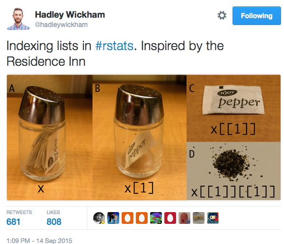
• Keep in mind the difference between the following:
  • Extracting a data frame’s variable (column) in itself, as a vector (numeric, character, etc.) — The single pepper packet by itself in the figure below (panel C). This is given by df[[i]], df[["variable.name"]], df$variable.name.
  • Extracting another data frame of just one variable (column) – The single pepper packet within the pepper shaker in the figure below (panel B). This is given by df[i], df["variable.name"].
• Subsetting verbs in tidyverse. In addition to subsetting data frames via the base indexing syntax described above, we can also use the subsetting functions introduced by the dplyr package in tidyverse (see below).

# Numeric subsetting                                                          ----
# - - - - - - - - - - - - - - - - - - - - - - - - - - - - - - - - - - - - - - - 

# Let's use our vector of ego age values again.
age

##  [1] 61 38 30 25 29 56 52 35 22 51

# Index its 2nd element: The age of the 2nd respondent.
age[2]

## [1] 38

# Its 2nd, 4th and 5th elements.
age[c(2,4,5)]

## [1] 38 25 29

# Fifth to seventh elements
age[5:7]

## [1] 29 56 52

# Use indexing to assign (replace) an element.
age[2] <- 45

# The content of x has now changed.
age

##  [1] 61 45 30 25 29 56 52 35 22 51

# Let's subset the adjacency matrix we created before.
adj

##      [,1] [,2] [,3]
## [1,]    0    1    1
## [2,]    1    0    1
## [3,]    0    0    0

# Its 2,3 cell: Edge from node 2 to node 3.
adj[2,3]

## [1] 1

# Its 2nd column: All edges to node 2.
adj[,2]

## [1] 1 0 0

# Its 2nd and 3rd row: All edges from nodes 2 and 3.
adj[2:3,]

##      [,1] [,2] [,3]
## [1,]    1    0    1
## [2,]    0    0    0

# Logical subsetting                                                          ----
# - - - - - - - - - - - - - - - - - - - - - - - - - - - - - - - - - - - - - - - 

# Which values of "age" are between 40 and 60?

# Let's create a logical index that flags these values.
(ind <- age > 40 & age < 60)

##  [1] FALSE  TRUE FALSE FALSE FALSE  TRUE  TRUE FALSE FALSE  TRUE

# Use this index to extract these values from vector "age" via logical subsetting.
age[ind]

## [1] 45 56 52 51

# We could also have typed directly:
age[age > 40 & age < 60]

## [1] 45 56 52 51

# Subsetting data frames                                                     ---- 
# - - - - - - - - - - - - - - - - - - - - - - - - - - - - - - - - - - - - - - - 

# We'll use our ego-level data frame.
ego.df

## # A tibble: 102 × 9
##    ego_ID ego.sex ego.age ego.arr ego.edu ego.inc  empl ego.empl.bin ego.age.cat
##     <dbl> <chr>     <dbl>   <dbl> <chr>     <dbl> <dbl> <chr>        <chr>      
##  1     28 Male         61    2008 Second…     350     3 Yes          60+        
##  2     29 Male         38    2000 Primary     900     4 Yes          36-40      
##  3     33 Male         30    2010 Primary     200     3 Yes          26-30      
##  4     35 Male         25    2009 Second…    1000     3 Yes          18-25      
##  5     39 Male         29    2007 Primary       0     1 No           26-30      
##  6     40 Male         56    2008 Second…     950     4 Yes          51-60      
##  7     45 Male         52    1975 Primary    1600     3 Yes          51-60      
##  8     46 Male         35    2002 Second…    1200     4 Yes          31-35      
##  9     47 Male         22    2010 Second…     700     4 Yes          18-25      
## 10     48 Male         51    2007 Primary     950     4 Yes          51-60      
## # ℹ 92 more rows

# Numeric subsetting works on data frames too: it allows you to index variables.

# The 3rd variable.
ego.df[3]

## # A tibble: 102 × 1
##    ego.age
##      <dbl>
##  1      61
##  2      38
##  3      30
##  4      25
##  5      29
##  6      56
##  7      52
##  8      35
##  9      22
## 10      51
## # ℹ 92 more rows

# Note the difference with the double square bracket.
ego.df[[3]]

##   [1] 61 38 30 25 29 56 52 35 22 51 50 45 51 32 57 42 32 55 44 25 28 60 54 30 37
##  [26] 41 47 33 37 29 39 31 52 30 57 44 47 42 44 31 31 56 36 47 47 35 43 22 55 32
##  [51] NA 60 51 53 25 33 38 37 27 34 32 26 36 53 42 45 36 54 49 35 27 32 58 51 55
##  [76] 59 27 35 24 52 27 42 47 43 53 54 35 50 51 40 49 33 33 36 32 35 55 61 34 44
## [101] 50 28

# What do you think is the difference?
class(ego.df[3])

## [1] "tbl_df"     "tbl"        "data.frame"

class(ego.df[[3]])

## [1] "numeric"

# The [[ ]] notation extracts the actual column as a vector, while [ ] keeps
# the data frame class.

# We can also subset data frames as matrices.
# The second and third columns.
ego.df[,2:3]

## # A tibble: 102 × 2
##    ego.sex ego.age
##    <chr>     <dbl>
##  1 Male         61
##  2 Male         38
##  3 Male         30
##  4 Male         25
##  5 Male         29
##  6 Male         56
##  7 Male         52
##  8 Male         35
##  9 Male         22
## 10 Male         51
## # ℹ 92 more rows

# Lines 1 to 3
ego.df[1:3,]

## # A tibble: 3 × 9
##   ego_ID ego.sex ego.age ego.arr ego.edu  ego.inc  empl ego.empl.bin ego.age.cat
##    <dbl> <chr>     <dbl>   <dbl> <chr>      <dbl> <dbl> <chr>        <chr>      
## 1     28 Male         61    2008 Seconda…     350     3 Yes          60+        
## 2     29 Male         38    2000 Primary      900     4 Yes          36-40      
## 3     33 Male         30    2010 Primary      200     3 Yes          26-30

# We can use name indexing with data frames, selecting variables by name
ego.df["ego.age"]

## # A tibble: 102 × 1
##    ego.age
##      <dbl>
##  1      61
##  2      38
##  3      30
##  4      25
##  5      29
##  6      56
##  7      52
##  8      35
##  9      22
## 10      51
## # ℹ 92 more rows

ego.df[["ego.age"]]

##   [1] 61 38 30 25 29 56 52 35 22 51 50 45 51 32 57 42 32 55 44 25 28 60 54 30 37
##  [26] 41 47 33 37 29 39 31 52 30 57 44 47 42 44 31 31 56 36 47 47 35 43 22 55 32
##  [51] NA 60 51 53 25 33 38 37 27 34 32 26 36 53 42 45 36 54 49 35 27 32 58 51 55
##  [76] 59 27 35 24 52 27 42 47 43 53 54 35 50 51 40 49 33 33 36 32 35 55 61 34 44
## [101] 50 28

# The $ notation is very common and concise. It's equivalent to the [[ notation.
ego.df$ego.age

##   [1] 61 38 30 25 29 56 52 35 22 51 50 45 51 32 57 42 32 55 44 25 28 60 54 30 37
##  [26] 41 47 33 37 29 39 31 52 30 57 44 47 42 44 31 31 56 36 47 47 35 43 22 55 32
##  [51] NA 60 51 53 25 33 38 37 27 34 32 26 36 53 42 45 36 54 49 35 27 32 58 51 55
##  [76] 59 27 35 24 52 27 42 47 43 53 54 35 50 51 40 49 33 33 36 32 35 55 61 34 44
## [101] 50 28

# This is the same as ego.df[[3]] or ego.df[["ego.age"]]
identical(ego.df[[3]], ego.df$ego.age)

## [1] TRUE

# With tidyverse, this type of subsetting syntax is replaced by new "verbs" 
# (see section below):
# * Index data frame rows: filter() instead of []
# * Index data frame columns: select() instead of []
# * Extract data frame variable as a vector: pull() instead of [[]] or $


# ***** EXERCISES 
#
# (1) What's the mean age of respondents whose education is NOT "Primary"? Use
# the ego.age and ego.edu variables. Remember that the "different from"
# comparison operator is !=.
#
# (2) What is the modal education level (i.e., the most common education level)
# of respondents who are older than 40? Use table() or tabyl().
#
# (3) Create the fictitious variable var <- c(1:30, rep(NA, 3), 34:50). Use is.na()
# to index all the NA values in the variable. Then use is.na() to index all
# values that are *not* NA. Hint: Remember the operator used to negate a logical
# vector. Finally, use this indexing to remove all NA values from var.
#
# (4) Use the $ notation to extract the "ego.arr" variable in ego.df. Recode all 
# values equal to 2008 as 99. Hint: Index all values equal to 2008, then replace 
# them with 99 via the assignment operator. 
#
# *****

2.6 The tidyverse syntax

2.6.1 Pipes and the |> operator

• The original pipe operator, %>%, was introduced by the magrittr package in 2014. It quickly gained popularity in the R community and was adopted by igraph and tidyverse (among other packages), which we use in this workshop. In 2021, R incorporated the pipe idea with a new, similar (but not identical) operator: |>. See this page for an overview of the differences between |> and %>%.
• The idea behind pipes is in essence very simple:
  • f(g(x)) becomes x |> g() |> f().
  • For example: mean(table(x)) becomes x |> table() |> mean().
• So |> pipes the output of the previous function (e.g., table()) into the input of the following function (e.g., mean()). This turns inside-to-outside code into left-to-right code. Because left to right is the direction most of us are used to read in (at least in English and other Western languages), pipes make R code easier to read and follow.
• You may also see pipes concatenating multiple lines of code. That’s possible and a common coding style. Instead of

x |> table() |> mean()

you can write

x |>
  table() |>
  mean()

2.6.2 Subsetting data frames in tidyverse

• Tidyverse includes the dplyr package for data frame manipulation. This is a very powerful package for all kinds of data wrangling. To learn more, see the package cheatsheet and vignettes.
• Subsetting data frames with dplyr:
  • dplyr::filter() is used to subset rows (cases) of a data frame based on one or multiple conditions (for example, respondents with certain values on one or more variables). This preserves the data frame class, similar to [ ] indexing.
  • dplyr::select() is used to subset columns (variables) of a data frame. You can use full variable names or select variables in many other ways (see examples in the select manual page). This preserves the data frame class, similar to [ ] indexing.
  • dplyr::pull() is used to extract a column as a vector. This does not preserve the data frame class, similar to [[ ]] or $.

# The pipe operator                                                         ----
# - - - - - - - - - - - - - - - - - - - - - - - - - - - - - - - - - - - - - - - 

# Ego education variable 
(edu <- ego.df$ego.edu)

##   [1] "Secondary"  "Primary"    "Primary"    "Secondary"  "Primary"   
##   [6] "Secondary"  "Primary"    "Secondary"  "Secondary"  "Primary"   
##  [11] "Secondary"  "Secondary"  "University" "Primary"    "Secondary" 
##  [16] "Primary"    "Primary"    "Secondary"  "Secondary"  "Primary"   
##  [21] "University" "University" "Primary"    "Secondary"  "Primary"   
##  [26] "Primary"    "Secondary"  "Primary"    "Primary"    "Primary"   
##  [31] "Secondary"  "Secondary"  "Secondary"  "Primary"    "Primary"   
##  [36] "Secondary"  "Secondary"  "Primary"    "Secondary"  "Primary"   
##  [41] "Primary"    "Primary"    "Primary"    "Secondary"  "Primary"   
##  [46] "Primary"    "Primary"    "University" "Primary"    "Secondary" 
##  [51] "University" "Primary"    "University" "Secondary"  "Secondary" 
##  [56] "University" "Primary"    "Primary"    "Secondary"  "Secondary" 
##  [61] "Secondary"  "University" "University" "University" "Secondary" 
##  [66] "Secondary"  "Secondary"  "University" "Primary"    "Secondary" 
##  [71] "Secondary"  "Secondary"  "University" "Primary"    "Secondary" 
##  [76] "Secondary"  "Secondary"  "Secondary"  "Secondary"  "Secondary" 
##  [81] "Secondary"  "Primary"    "Primary"    "University" "Primary"   
##  [86] "Primary"    "Secondary"  "Secondary"  "Secondary"  "University"
##  [91] "Secondary"  "Secondary"  "Primary"    "Primary"    "University"
##  [96] "Primary"    "Primary"    "Primary"    "Primary"    "Secondary" 
## [101] "Primary"    "Secondary"

# Frequency of educational categories in the data
table(edu)

## edu
##    Primary  Secondary University 
##         42         45         15

# Average frequency
mean(table(edu))

## [1] 34

# Let's re-write this with the pipe operator
edu |> 
  table() |> 
  mean()

## [1] 34

# Subsetting data frames with dplyr: filter and select                      ----
# - - - - - - - - - - - - - - - - - - - - - - - - - - - - - - - - - - - - - - - 

# Filter to egos who are older than 40
ego.df |> 
  filter(ego.age > 40)

## # A tibble: 51 × 9
##    ego_ID ego.sex ego.age ego.arr ego.edu ego.inc  empl ego.empl.bin ego.age.cat
##     <dbl> <chr>     <dbl>   <dbl> <chr>     <dbl> <dbl> <chr>        <chr>      
##  1     28 Male         61    2008 Second…     350     3 Yes          60+        
##  2     40 Male         56    2008 Second…     950     4 Yes          51-60      
##  3     45 Male         52    1975 Primary    1600     3 Yes          51-60      
##  4     48 Male         51    2007 Primary     950     4 Yes          51-60      
##  5     49 Male         50    2001 Second…    1300     4 Yes          41-50      
##  6     51 Male         45    2011 Second…     480     3 Yes          41-50      
##  7     52 Male         51    2002 Univer…    1200     4 Yes          51-60      
##  8     55 Male         57    1979 Second…     470     7 No           51-60      
##  9     56 Male         42    1992 Primary    1100     4 Yes          41-50      
## 10     58 Male         55    1990 Second…    1450     4 Yes          51-60      
## # ℹ 41 more rows

# Filter to egos with Primary education
ego.df |> 
  filter(ego.edu == "Primary")

## # A tibble: 42 × 9
##    ego_ID ego.sex ego.age ego.arr ego.edu ego.inc  empl ego.empl.bin ego.age.cat
##     <dbl> <chr>     <dbl>   <dbl> <chr>     <dbl> <dbl> <chr>        <chr>      
##  1     29 Male         38    2000 Primary     900     4 Yes          36-40      
##  2     33 Male         30    2010 Primary     200     3 Yes          26-30      
##  3     39 Male         29    2007 Primary       0     1 No           26-30      
##  4     45 Male         52    1975 Primary    1600     3 Yes          51-60      
##  5     48 Male         51    2007 Primary     950     4 Yes          51-60      
##  6     53 Male         32    2003 Primary    1600     1 No           31-35      
##  7     56 Male         42    1992 Primary    1100     4 Yes          41-50      
##  8     57 Male         32    2000 Primary    1200     4 Yes          31-35      
##  9     60 Male         25    2011 Primary       0     1 No           18-25      
## 10     64 Male         54    1981 Primary     300     3 Yes          51-60      
## # ℹ 32 more rows

# Combine the two conditions: Intersection.
ego.df |> 
  filter(ego.age > 40 & ego.edu == "Primary")

## # A tibble: 21 × 9
##    ego_ID ego.sex ego.age ego.arr ego.edu ego.inc  empl ego.empl.bin ego.age.cat
##     <dbl> <chr>     <dbl>   <dbl> <chr>     <dbl> <dbl> <chr>        <chr>      
##  1     45 Male         52    1975 Primary    1600     3 Yes          51-60      
##  2     48 Male         51    2007 Primary     950     4 Yes          51-60      
##  3     56 Male         42    1992 Primary    1100     4 Yes          41-50      
##  4     64 Male         54    1981 Primary     300     3 Yes          51-60      
##  5     68 Male         41    2008 Primary     600     4 Yes          41-50      
##  6     82 Male         57    1982 Primary    1190     4 Yes          51-60      
##  7     85 Male         42    2008 Primary     400     2 No           41-50      
##  8     90 Male         56    2004 Primary     450     4 Yes          51-60      
##  9     93 Male         47    2010 Primary     880     4 Yes          41-50      
## 10     95 Male         43    1997 Primary     800     4 Yes          41-50      
## # ℹ 11 more rows

# Combine the two conditions: Union.
ego.df |> 
  filter(ego.age > 40 | ego.edu == "Primary")

## # A tibble: 72 × 9
##    ego_ID ego.sex ego.age ego.arr ego.edu ego.inc  empl ego.empl.bin ego.age.cat
##     <dbl> <chr>     <dbl>   <dbl> <chr>     <dbl> <dbl> <chr>        <chr>      
##  1     28 Male         61    2008 Second…     350     3 Yes          60+        
##  2     29 Male         38    2000 Primary     900     4 Yes          36-40      
##  3     33 Male         30    2010 Primary     200     3 Yes          26-30      
##  4     39 Male         29    2007 Primary       0     1 No           26-30      
##  5     40 Male         56    2008 Second…     950     4 Yes          51-60      
##  6     45 Male         52    1975 Primary    1600     3 Yes          51-60      
##  7     48 Male         51    2007 Primary     950     4 Yes          51-60      
##  8     49 Male         50    2001 Second…    1300     4 Yes          41-50      
##  9     51 Male         45    2011 Second…     480     3 Yes          41-50      
## 10     52 Male         51    2002 Univer…    1200     4 Yes          51-60      
## # ℹ 62 more rows

# Note that the object ego.df hasn't changed. To re-use any of the filtered data
# frames above, we have to assign them to an object.
ego.df.40 <- ego.df |> 
  filter(ego.age > 40)

ego.df.40

## # A tibble: 51 × 9
##    ego_ID ego.sex ego.age ego.arr ego.edu ego.inc  empl ego.empl.bin ego.age.cat
##     <dbl> <chr>     <dbl>   <dbl> <chr>     <dbl> <dbl> <chr>        <chr>      
##  1     28 Male         61    2008 Second…     350     3 Yes          60+        
##  2     40 Male         56    2008 Second…     950     4 Yes          51-60      
##  3     45 Male         52    1975 Primary    1600     3 Yes          51-60      
##  4     48 Male         51    2007 Primary     950     4 Yes          51-60      
##  5     49 Male         50    2001 Second…    1300     4 Yes          41-50      
##  6     51 Male         45    2011 Second…     480     3 Yes          41-50      
##  7     52 Male         51    2002 Univer…    1200     4 Yes          51-60      
##  8     55 Male         57    1979 Second…     470     7 No           51-60      
##  9     56 Male         42    1992 Primary    1100     4 Yes          41-50      
## 10     58 Male         55    1990 Second…    1450     4 Yes          51-60      
## # ℹ 41 more rows

# Select specific variables
ego.df.40 |>
  dplyr::select(ego.sex, ego.age)

## # A tibble: 51 × 2
##    ego.sex ego.age
##    <chr>     <dbl>
##  1 Male         61
##  2 Male         56
##  3 Male         52
##  4 Male         51
##  5 Male         50
##  6 Male         45
##  7 Male         51
##  8 Male         57
##  9 Male         42
## 10 Male         55
## # ℹ 41 more rows

# As usual, we can re-assign the result to the same data object
ego.df.40 <- ego.df.40 |> 
  dplyr::select(ego.sex, ego.age)

ego.df.40

## # A tibble: 51 × 2
##    ego.sex ego.age
##    <chr>     <dbl>
##  1 Male         61
##  2 Male         56
##  3 Male         52
##  4 Male         51
##  5 Male         50
##  6 Male         45
##  7 Male         51
##  8 Male         57
##  9 Male         42
## 10 Male         55
## # ℹ 41 more rows

# Pull a variable out of a data frame, as a vector
ego.df |>
  pull(ego.age)

##   [1] 61 38 30 25 29 56 52 35 22 51 50 45 51 32 57 42 32 55 44 25 28 60 54 30 37
##  [26] 41 47 33 37 29 39 31 52 30 57 44 47 42 44 31 31 56 36 47 47 35 43 22 55 32
##  [51] NA 60 51 53 25 33 38 37 27 34 32 26 36 53 42 45 36 54 49 35 27 32 58 51 55
##  [76] 59 27 35 24 52 27 42 47 43 53 54 35 50 51 40 49 33 33 36 32 35 55 61 34 44
## [101] 50 28

# This is the same as
ego.df$ego.age

##   [1] 61 38 30 25 29 56 52 35 22 51 50 45 51 32 57 42 32 55 44 25 28 60 54 30 37
##  [26] 41 47 33 37 29 39 31 52 30 57 44 47 42 44 31 31 56 36 47 47 35 43 22 55 32
##  [51] NA 60 51 53 25 33 38 37 27 34 32 26 36 53 42 45 36 54 49 35 27 32 58 51 55
##  [76] 59 27 35 24 52 27 42 47 43 53 54 35 50 51 40 49 33 33 36 32 35 55 61 34 44
## [101] 50 28

# ***** EXERCISES 
#
# (1) Use the [ , ] notation to extract the education level and income of egos who
# are younger than 30. Then do the same thing with the dplyr::filter() function.
# 
# *****