Chapter 6 Multilevel modeling of ego-network data

In progress.

6.1 Resources

6.1.1 Multilevel models for egocentric network data

Specific resources on multilevel modeling of egocentric/personal network data:

Vacca (2018): overview of multilevel modeling for egocentric/personal network data, with R demo (the code below is drawn in part from this article).
Duijn (2013): overview of multilevel modeling for egocentric and sociocentric data.
Vacca et al. (2019): multilevel models for overlapping egocentric networks.
McCarty et al. (2019): Ch. 13.
Perry et al. (2018): Ch. 8.
Crossley et al. (2015): Ch. 6.

6.1.2 Multilevel modeling in general

General resources on multilevel models:

Rasbash et al. (2008): Extensive online course on multilevel modeling for the social sciences, including Stata and R implementation.
Snijders & Bosker (2012): mode in-depth statistical treatment, social science focus.
Goldstein (2010)
Fox & Weisberg (2018): Ch. 7, R implementation with lme4.
GLMM FAQ by Ben Bolker and others: online list of R packages and resources on linear and generalized linear mixed models.

6.2 Prepare the data

# Load packages.
library(tidyverse)
library(lme4)
library(car)
library(skimr)
library(janitor)
library(broom.mixed)

# Clear the workspace from all previous objects
rm(list=ls())

# Load the data
load("./Data/data.rda")

# Create data frame object for models (level-1 join)
(model.data <- left_join(alter.attr.all, ego.df, by= "ego_ID"))

## # A tibble: 4,590 × 20
##    alter_ID ego_ID alter_num alter.sex alter.age.cat alter.rel    alter.nat
##       <dbl>  <dbl>     <dbl> <fct>     <fct>         <fct>        <fct>    
##  1     2801     28         1 Female    51-60         Close family Sri Lanka
##  2     2802     28         2 Male      51-60         Other family Sri Lanka
##  3     2803     28         3 Male      51-60         Close family Sri Lanka
##  4     2804     28         4 Male      60+           Close family Sri Lanka
##  5     2805     28         5 Female    41-50         Close family Sri Lanka
##  6     2806     28         6 Female    60+           Close family Sri Lanka
##  7     2807     28         7 Male      41-50         Other family Sri Lanka
##  8     2808     28         8 Female    36-40         Other family Sri Lanka
##  9     2809     28         9 Female    51-60         Other family Sri Lanka
## 10     2810     28        10 Male      60+           Other family Sri Lanka
## # ℹ 4,580 more rows
## # ℹ 13 more variables: alter.res <fct>, alter.clo <dbl>, alter.loan <fct>,
## #   alter.fam <fct>, alter.age <dbl>, ego.sex <fct>, ego.age <dbl>,
## #   ego.arr <dbl>, ego.edu <fct>, ego.inc <dbl>, empl <dbl>,
## #   ego.empl.bin <fct>, ego.age.cat <fct>

## Create variables to be used in multilevel models                         ====
# ============================================================================ =

# Ego-alter age homophily variable
# - - - - - - - - - - - - - - - - - 

# (TRUE if alter and ego are in the same age bracket)
model.data <- model.data |>  
  mutate(alter.same.age = (alter.age.cat==ego.age.cat))  

# See result
tabyl(model.data$alter.same.age)

##  model.data$alter.same.age    n    percent valid_percent
##                      FALSE 3228 0.70326797     0.7113266
##                       TRUE 1310 0.28540305     0.2886734
##                         NA   52 0.01132898            NA

# Recode: TRUE = Yes, FALSE = No
model.data <- model.data |> 
  mutate(alter.same.age = as.character(alter.same.age),
         alter.same.age = fct_recode(alter.same.age,
                                     Yes = "TRUE", No = "FALSE"))

# See result
tabyl(model.data$alter.same.age)

##  model.data$alter.same.age    n    percent valid_percent
##                         No 3228 0.70326797     0.7113266
##                        Yes 1310 0.28540305     0.2886734
##                       <NA>   52 0.01132898            NA

# Centered/rescaled versions of ego and alter age 
# - - - - - - - - - - - - - - - - - - - - - - - - 

# This is done for easier interpretation of model coefficients
model.data <- model.data |> 
  # Ego age centered around its mean and scaled by 5 (1 unit = 5 years)
  mutate(ego.age.cen = scale(ego.age, scale= 5),
         # Alter age category centered around its mean
         alter.age.cat.cen = scale(as.numeric(alter.age.cat), scale= FALSE))

# Count of family members in ego-network
# - - - - - - - - - - - - - - - - - - - - - - - - 

model.data <- model.data |> 
  group_by(ego_ID) |>
  mutate(net.count.fam = sum(alter.fam=="Yes", na.rm=TRUE)) |>
  ungroup()

# Center and rescale by 5 (+1 unit = 5 more family members in ego-network)
model.data <- model.data |> 
  mutate(net.count.fam.cen = scale(net.count.fam, scale=5))

6.3 Random intercept models

## m1: Variance components models                                           ====
# ============================================================================ =

# Variance components model: level 1 is ties, level 2 is egos, random intercept, 
# no predictor
m1 <- glmer(alter.loan ~ # Dependent variable
              (1 | ego_ID), # Intercept (1) varies in level-2 units (ego_ID)
            family = binomial("logit"), # Model class (logistic)
            data = model.data) # Data object

# View results
car::S(m1)

## Generalized linear mixed model fit by ML
## Call: glmer(formula = alter.loan ~ (1 | ego_ID), data = model.data, family =
##             binomial("logit"))
## 
## Estimates of Fixed Effects:
##             Estimate Std. Error z value Pr(>|z|)
## (Intercept)  0.05376    0.09609   0.559    0.576
## 
## Exponentiated Fixed Effects and Confidence Bounds:
##             Estimate     2.5 %   97.5 %
## (Intercept) 1.055234 0.8740859 1.273925
## 
## Estimates of Random Effects (Covariance Components):
##  Groups Name        Std.Dev.
##  ego_ID (Intercept) 0.9001  
## 
## Number of obs: 4021, groups:  ego_ID, 101
## 
##   logLik       df      AIC      BIC 
## -2577.23        2  5158.46  5171.06

## m2: Add tie characteristics as predictors (level 1)                      ====
# ============================================================================ =

# Add alter.fam and alter.same.age as predictors

# See descriptives for the new predictors
tabyl(model.data$alter.fam)

##  model.data$alter.fam    n   percent
##                    No 3202 0.6976035
##                   Yes 1388 0.3023965

tabyl(model.data$alter.same.age)

##  model.data$alter.same.age    n    percent valid_percent
##                         No 3228 0.70326797     0.7113266
##                        Yes 1310 0.28540305     0.2886734
##                       <NA>   52 0.01132898            NA

# Estimate the model and view results
m2 <- glmer(alter.loan ~ # Dependent variable
              alter.fam + alter.same.age + # Tie characteristics
              (1 | ego_ID), # Intercept (1) varies in level-2 units (ego_ID)
            family = binomial("logit"), # Model class (logistic)
            data = model.data) # Data object
car::S(m2)

## Generalized linear mixed model fit by ML
## Call: glmer(formula = alter.loan ~ alter.fam + alter.same.age + (1 | ego_ID),
##             data = model.data, family = binomial("logit"))
## 
## Estimates of Fixed Effects:
##                   Estimate Std. Error z value Pr(>|z|)    
## (Intercept)       -0.21556    0.10511  -2.051   0.0403 *  
## alter.famYes       1.01248    0.09284  10.906   <2e-16 ***
## alter.same.ageYes  0.20385    0.07951   2.564   0.0104 *  
## ---
## Signif. codes:  0 '***' 0.001 '**' 0.01 '*' 0.05 '.' 0.1 ' ' 1
## 
## Exponentiated Fixed Effects and Confidence Bounds:
##                   Estimate     2.5 %    97.5 %
## (Intercept)       0.806089 0.6560166 0.9904925
## alter.famYes      2.752416 2.2945237 3.3016850
## alter.same.ageYes 1.226113 1.0491868 1.4328735
## 
## Estimates of Random Effects (Covariance Components):
##  Groups Name        Std.Dev.
##  ego_ID (Intercept) 0.9372  
## 
## Number of obs: 3972, groups:  ego_ID, 100
## 
##   logLik       df      AIC      BIC 
## -2478.16        4  4964.31  4989.46

## m3: Add ego characteristics as predictors (level 2)                      ====
# ============================================================================ =

# Add ego age (ego.age.cen), employment status (ego.empl.bin), 
# educational level (ego.edu)

# See descriptives for the new predictors
skim_tee(model.data$ego.age.cen)

## ── Data Summary ────────────────────────
##                            Values
## Name                       data  
## Number of rows             4590  
## Number of columns          1     
## _______________________          
## Column type frequency:           
##   numeric                  1     
## ________________________         
## Group variables            None  
## 
## ── Variable type: numeric ──────────────────────────────────────────────────────
##   skim_variable n_missing complete_rate     mean   sd    p0   p25     p50  p75
## 1 V1                   45         0.990 1.09e-15 2.14 -3.85 -1.85 -0.0515 1.95
##   p100 hist 
## 1 3.95 ▃▇▅▆▅

tabyl(model.data$ego.empl.bin)

##  model.data$ego.empl.bin    n   percent
##                       No  900 0.1960784
##                      Yes 3690 0.8039216

tabyl(model.data$ego.edu)

##  model.data$ego.edu    n   percent
##             Primary 1890 0.4117647
##           Secondary 2025 0.4411765
##          University  675 0.1470588

# Estimate the model and view results
m3 <- glmer(alter.loan ~ alter.fam + alter.same.age + # Tie characteristics
              ego.age.cen + ego.empl.bin + ego.edu + # Ego characteristics
              (1 | ego_ID), # Intercept (1) varies in level-2 units
            family = binomial("logit"), # Model class (logistic)
            data = model.data) # Data
car::S(m3)

## Generalized linear mixed model fit by ML
## Call: glmer(formula = alter.loan ~ alter.fam + alter.same.age + ego.age.cen +
##             ego.empl.bin + ego.edu + (1 | ego_ID), data = model.data, family =
##             binomial("logit"))
## 
## Estimates of Fixed Effects:
##                   Estimate Std. Error z value Pr(>|z|)    
## (Intercept)       -0.61436    0.22536  -2.726  0.00641 ** 
## alter.famYes       1.00698    0.09285  10.845  < 2e-16 ***
## alter.same.ageYes  0.19790    0.07950   2.489  0.01281 *  
## ego.age.cen       -0.01306    0.04487  -0.291  0.77099    
## ego.empl.binYes    0.07830    0.24563   0.319  0.74991    
## ego.eduSecondary   0.49402    0.20962   2.357  0.01844 *  
## ego.eduUniversity  0.86482    0.29947   2.888  0.00388 ** 
## ---
## Signif. codes:  0 '***' 0.001 '**' 0.01 '*' 0.05 '.' 0.1 ' ' 1
## 
## Exponentiated Fixed Effects and Confidence Bounds:
##                    Estimate     2.5 %    97.5 %
## (Intercept)       0.5409892 0.3478234 0.8414306
## alter.famYes      2.7373325 2.2818749 3.2836986
## alter.same.ageYes 1.2188387 1.0429695 1.4243637
## ego.age.cen       0.9870230 0.9039204 1.0777658
## ego.empl.binYes   1.0814450 0.6682212 1.7502037
## ego.eduSecondary  1.6388905 1.0867238 2.4716141
## ego.eduUniversity 2.3745730 1.3202994 4.2706956
## 
## Estimates of Random Effects (Covariance Components):
##  Groups Name        Std.Dev.
##  ego_ID (Intercept) 0.879   
## 
## Number of obs: 3972, groups:  ego_ID, 100
## 
##   logLik       df      AIC      BIC 
## -2472.68        8  4961.36  5011.66

## m4: Add alter characteristics as predictors (level 1)                        ====
# ============================================================================ =

# Add alter sex and alter age (centered)

# See descriptives for the new predictors
tabyl(model.data$alter.sex)

##  model.data$alter.sex    n   percent
##                Female 1297 0.2825708
##                  Male 3293 0.7174292

skim_tee(model.data$alter.age.cat.cen)

## ── Data Summary ────────────────────────
##                            Values
## Name                       data  
## Number of rows             4590  
## Number of columns          1     
## _______________________          
## Column type frequency:           
##   numeric                  1     
## ________________________         
## Group variables            None  
## 
## ── Variable type: numeric ──────────────────────────────────────────────────────
##   skim_variable n_missing complete_rate     mean   sd    p0   p25    p50   p75
## 1 V1                    8         0.998 1.95e-15 1.64 -3.13 -1.13 -0.126 0.874
##   p100 hist 
## 1 2.87 ▆▅▆▇▆

# Estimate the model and view results
m4 <- glmer(alter.loan ~ alter.fam + alter.same.age + # Tie characteristics
              ego.age.cen + ego.empl.bin + ego.edu + # Ego characteristics
              alter.sex + alter.age.cat.cen + # Alter characteristics
              (1 | ego_ID), # Intercept (1) varies in level-2 units
            family = binomial("logit"), # Model class (logistic)
            data= model.data) # Data
car::S(m4)

## Generalized linear mixed model fit by ML
## Call: glmer(formula = alter.loan ~ alter.fam + alter.same.age + ego.age.cen +
##             ego.empl.bin + ego.edu + alter.sex + alter.age.cat.cen + (1 | ego_ID), data =
##             model.data, family = binomial("logit"))
## 
## Estimates of Fixed Effects:
##                   Estimate Std. Error z value Pr(>|z|)    
## (Intercept)       -0.79887    0.23618  -3.383 0.000718 ***
## alter.famYes       1.04455    0.09450  11.053  < 2e-16 ***
## alter.same.ageYes  0.18047    0.07984   2.261 0.023786 *  
## ego.age.cen       -0.02345    0.04544  -0.516 0.605772    
## ego.empl.binYes    0.06895    0.24628   0.280 0.779486    
## ego.eduSecondary   0.49039    0.21008   2.334 0.019578 *  
## ego.eduUniversity  0.87968    0.30013   2.931 0.003379 ** 
## alter.sexMale      0.25266    0.08596   2.939 0.003289 ** 
## alter.age.cat.cen  0.03834    0.02475   1.549 0.121300    
## ---
## Signif. codes:  0 '***' 0.001 '**' 0.01 '*' 0.05 '.' 0.1 ' ' 1
## 
## Exponentiated Fixed Effects and Confidence Bounds:
##                    Estimate     2.5 %    97.5 %
## (Intercept)       0.4498365 0.2831526 0.7146425
## alter.famYes      2.8421300 2.3615731 3.4204755
## alter.same.ageYes 1.1977844 1.0242887 1.4006672
## ego.age.cen       0.9768214 0.8935895 1.0678058
## ego.empl.binYes   1.0713874 0.6611755 1.7361061
## ego.eduSecondary  1.6329480 1.0818205 2.4648443
## ego.eduUniversity 2.4101365 1.3383500 4.3402381
## alter.sexMale     1.2874404 1.0878274 1.5236817
## alter.age.cat.cen 1.0390877 0.9898894 1.0907312
## 
## Estimates of Random Effects (Covariance Components):
##  Groups Name        Std.Dev.
##  ego_ID (Intercept) 0.881   
## 
## Number of obs: 3972, groups:  ego_ID, 100
## 
##   logLik       df      AIC      BIC 
## -2467.02       10  4954.04  5016.91

## m5: Add network characteristics as predictors (level 2)                  ====
# ============================================================================ =

# Add count of family members in network (centered)

# See descriptives for the new predictor
skim_tee(model.data$net.count.fam.cen)

## ── Data Summary ────────────────────────
##                            Values
## Name                       data  
## Number of rows             4590  
## Number of columns          1     
## _______________________          
## Column type frequency:           
##   numeric                  1     
## ________________________         
## Group variables            None  
## 
## ── Variable type: numeric ──────────────────────────────────────────────────────
##   skim_variable n_missing complete_rate     mean   sd    p0    p25    p50   p75
## 1 V1                    0             1 2.30e-16 1.02 -1.72 -0.722 -0.122 0.478
##   p100 hist 
## 1 2.88 ▃▇▅▂▁

# Estimate model and see results
m5 <- glmer(alter.loan ~ alter.fam + alter.same.age + # Tie characteristics
              ego.age.cen + ego.empl.bin + ego.edu + # Ego characteristics
              alter.sex + alter.age.cat.cen +  # Alter characteristics
              net.count.fam.cen + # Ego-network characteristics
              (1 | ego_ID), # Intercept (1) varies in level-2 units
            family = binomial("logit"), # Model class (logistic)
            data= model.data) # Data
car::S(m5)

## Generalized linear mixed model fit by ML
## Call: glmer(formula = alter.loan ~ alter.fam + alter.same.age + ego.age.cen +
##             ego.empl.bin + ego.edu + alter.sex + alter.age.cat.cen + net.count.fam.cen + (1
##             | ego_ID), data = model.data, family = binomial("logit"))
## 
## Estimates of Fixed Effects:
##                   Estimate Std. Error z value Pr(>|z|)    
## (Intercept)       -0.85010    0.23451  -3.625 0.000289 ***
## alter.famYes       1.06161    0.09498  11.178  < 2e-16 ***
## alter.same.ageYes  0.18265    0.07984   2.288 0.022143 *  
## ego.age.cen       -0.02294    0.04473  -0.513 0.608080    
## ego.empl.binYes    0.11925    0.24383   0.489 0.624801    
## ego.eduSecondary   0.49636    0.20680   2.400 0.016385 *  
## ego.eduUniversity  0.94460    0.29757   3.174 0.001502 ** 
## alter.sexMale      0.25065    0.08595   2.916 0.003544 ** 
## alter.age.cat.cen  0.03879    0.02474   1.568 0.116935    
## net.count.fam.cen -0.17863    0.09517  -1.877 0.060523 .  
## ---
## Signif. codes:  0 '***' 0.001 '**' 0.01 '*' 0.05 '.' 0.1 ' ' 1
## 
## Exponentiated Fixed Effects and Confidence Bounds:
##                    Estimate     2.5 %    97.5 %
## (Intercept)       0.4273712 0.2698904 0.6767418
## alter.famYes      2.8910105 2.3999717 3.4825169
## alter.same.ageYes 1.2003998 1.0265266 1.4037236
## ego.age.cen       0.9773249 0.8952995 1.0668653
## ego.empl.binYes   1.1266465 0.6986206 1.8169121
## ego.eduSecondary  1.6427235 1.0953169 2.4637077
## ego.eduUniversity 2.5717720 1.4352830 4.6081582
## alter.sexMale     1.2848651 1.0856573 1.5206256
## alter.age.cat.cen 1.0395482 0.9903442 1.0911968
## net.count.fam.cen 0.8364157 0.6940866 1.0079307
## 
## Estimates of Random Effects (Covariance Components):
##  Groups Name        Std.Dev.
##  ego_ID (Intercept) 0.8647  
## 
## Number of obs: 3972, groups:  ego_ID, 100
## 
##   logLik       df      AIC      BIC 
## -2465.28       11  4952.56  5021.72

# Results as tidy data frame
tidy(m5)

## # A tibble: 11 × 7
##    effect   group  term              estimate std.error statistic   p.value
##    <chr>    <chr>  <chr>                <dbl>     <dbl>     <dbl>     <dbl>
##  1 fixed    <NA>   (Intercept)        -0.850     0.235     -3.62   2.89e- 4
##  2 fixed    <NA>   alter.famYes        1.06      0.0950    11.2    5.25e-29
##  3 fixed    <NA>   alter.same.ageYes   0.183     0.0798     2.29   2.21e- 2
##  4 fixed    <NA>   ego.age.cen        -0.0229    0.0447    -0.513  6.08e- 1
##  5 fixed    <NA>   ego.empl.binYes     0.119     0.244      0.489  6.25e- 1
##  6 fixed    <NA>   ego.eduSecondary    0.496     0.207      2.40   1.64e- 2
##  7 fixed    <NA>   ego.eduUniversity   0.945     0.298      3.17   1.50e- 3
##  8 fixed    <NA>   alter.sexMale       0.251     0.0860     2.92   3.54e- 3
##  9 fixed    <NA>   alter.age.cat.cen   0.0388    0.0247     1.57   1.17e- 1
## 10 fixed    <NA>   net.count.fam.cen  -0.179     0.0952    -1.88   6.05e- 2
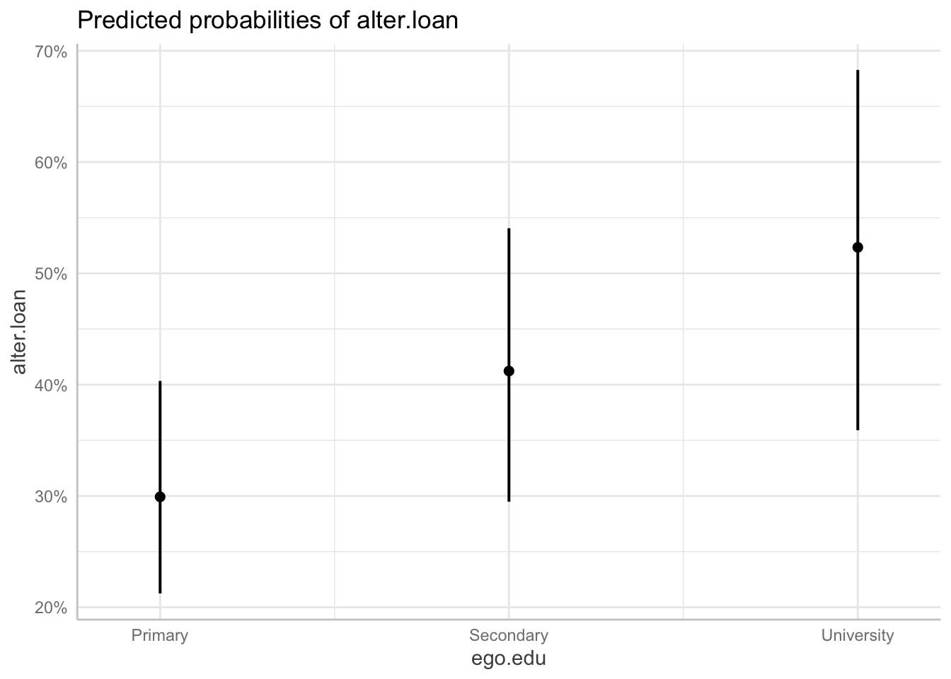
## 11 ran_pars ego_ID sd__(Intercept)     0.865    NA         NA     NA

## Plot predictor effects                                                   ====
# ============================================================================ =

library(ggeffects)

# Probability of financial support as a function of alter.fam
ggpredict(m5, "alter.fam")

## # Predicted probabilities of alter.loan
## 
## alter.fam | Predicted |       95% CI
## ------------------------------------
## No        |      0.30 | [0.21, 0.40]
## Yes       |      0.55 | [0.44, 0.66]
## 
## Adjusted for:
## *    alter.same.age =      No
## *       ego.age.cen =   -0.03
## *      ego.empl.bin =      No
## *           ego.edu = Primary
## *         alter.sex =  Female
## * alter.age.cat.cen =   -0.05
## * net.count.fam.cen =    0.00
## *            ego_ID = 0 (population-level)

# You can convert it to a tidy data frame
ggpredict(m5, "alter.fam") |>
  as_tibble()

## # A tibble: 2 × 6
##   x     predicted std.error conf.low conf.high group
##   <fct>     <dbl>     <dbl>    <dbl>     <dbl> <fct>
## 1 No        0.299     0.234    0.212     0.403 1    
## 2 Yes       0.552     0.239    0.436     0.66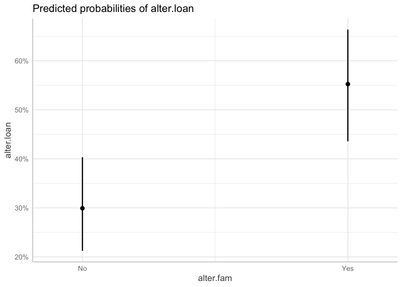4 1

# You can also plot the result
ggpredict(m5, "alter.fam") |> 
  plot()

# Probability of financial support as a function of ego.edu
ggpredict(m5, "ego.edu") |> 
  plot()

6.4 Random slope models

## m6: Random slope for alter.fam                                           ====
# ============================================================================ =

# Fit model
set.seed(2707)
m6 <- glmer(alter.loan ~ alter.fam + alter.same.age + # Tie characteristics
              ego.age.cen + ego.empl.bin + ego.edu + # Ego characteristics
              alter.sex + alter.age.cat.cen +  # Alter characteristics
              net.count.fam.cen + # Ego-network characteristics
              (1 + alter.fam | ego_ID), # Both intercept (1) and alter.fam 
            # slppe vary in level-2 units (ego_ID)
            family = binomial("logit"), # Model class (logistic)
            data = model.data) # Data

# Re-fit with starting values from previous fit to address convergence warnings

# Get estimate values from previous fit
ss <- getME(m6, c("theta", "fixef"))

# Refit by setting ss as starting values 
m6 <- glmer(alter.loan ~ alter.fam + alter.same.age + # Tie characteristics
              ego.age.cen + ego.empl.bin + ego.edu + # Ego characteristics
              alter.sex + alter.age.cat.cen +  # Alter characteristics
              net.count.fam.cen + # Ego-network characteristics
              (1 + alter.fam | ego_ID), # Both intercept (1) and alter.fam 
            start= ss, # 
            # slppe vary in level-2 units (ego_ID)
            family = binomial("logit"), # Model class (logistic)
            data= model.data) # Data

# View results
car::S(m6)

## Generalized linear mixed model fit by ML
## Call: glmer(formula = alter.loan ~ alter.fam + alter.same.age + ego.age.cen +
##             ego.empl.bin + ego.edu + alter.sex + alter.age.cat.cen + net.count.fam.cen + (1
##             + alter.fam | ego_ID), data = model.data, family = binomial("logit"), start =
##             ss)
## 
## Estimates of Fixed Effects:
##                   Estimate Std. Error z value Pr(>|z|)    
## (Intercept)       -0.91968    0.24605  -3.738 0.000186 ***
## alter.famYes       1.10130    0.12286   8.964  < 2e-16 ***
## alter.same.ageYes  0.18966    0.08067   2.351 0.018713 *  
## ego.age.cen       -0.02932    0.04559  -0.643 0.520114    
## ego.empl.binYes    0.16612    0.25192   0.659 0.509615    
## ego.eduSecondary   0.52521    0.21101   2.489 0.012809 *  
## ego.eduUniversity  1.00011    0.30744   3.253 0.001142 ** 
## alter.sexMale      0.25913    0.08691   2.982 0.002868 ** 
## alter.age.cat.cen  0.04229    0.02515   1.682 0.092584 .  
## net.count.fam.cen -0.18543    0.09693  -1.913 0.055745 .  
## ---
## Signif. codes:  0 '***' 0.001 '**' 0.01 '*' 0.05 '.' 0.1 ' ' 1
## 
## Exponentiated Fixed Effects and Confidence Bounds:
##                    Estimate     2.5 %    97.5 %
## (Intercept)       0.3986475 0.2461204 0.6456995
## alter.famYes      3.0080801 2.3643604 3.8270587
## alter.same.ageYes 1.2088406 1.0320627 1.4158981
## ego.age.cen       0.9711061 0.8881039 1.0618657
## ego.empl.binYes   1.1807181 0.7206342 1.9345392
## ego.eduSecondary  1.6908172 1.1181093 2.5568725
## ego.eduUniversity 2.7185746 1.4881625 4.9662908
## alter.sexMale     1.2958056 1.0928514 1.5364505
## alter.age.cat.cen 1.0432016 0.9930326 1.0959051
## net.count.fam.cen 0.8307445 0.6870036 1.0045601
## 
## Estimates of Random Effects (Covariance Components):
##  Groups Name         Std.Dev. Corr 
##  ego_ID (Intercept)  0.9054        
##         alter.famYes 0.6697   -0.27
## 
## Number of obs: 3972, groups:  ego_ID, 100
## 
##   logLik       df      AIC      BIC 
## -2460.22       13  4946.44  5028.17

# Results as tidy data frame
tidy(m6)

## # A tibble: 13 × 7
##    effect   group  term                   estimate std.error statistic   p.value
##    <chr>    <chr>  <chr>                     <dbl>     <dbl>     <dbl>     <dbl>
##  1 fixed    <NA>   (Intercept)             -0.920     0.246     -3.74   1.86e- 4
##  2 fixed    <NA>   alter.famYes             1.10      0.123      8.96   3.13e-19
##  3 fixed    <NA>   alter.same.ageYes        0.190     0.0807     2.35   1.87e- 2
##  4 fixed    <NA>   ego.age.cen             -0.0293    0.0456    -0.643  5.20e- 1
##  5 fixed    <NA>   ego.empl.binYes          0.166     0.252      0.659  5.10e- 1
##  6 fixed    <NA>   ego.eduSecondary         0.525     0.211      2.49   1.28e- 2
##  7 fixed    <NA>   ego.eduUniversity        1.00      0.307      3.25   1.14e- 3
##  8 fixed    <NA>   alter.sexMale            0.259     0.0869     2.98   2.87e- 3
##  9 fixed    <NA>   alter.age.cat.cen        0.0423    0.0251     1.68   9.26e- 2
## 10 fixed    <NA>   net.count.fam.cen       -0.185     0.0969    -1.91   5.57e- 2
## 11 ran_pars ego_ID sd__(Intercept)          0.905    NA         NA     NA       
## 12 ran_pars ego_ID cor__(Intercept).alte…  -0.275    NA         NA     NA       
## 13 ran_pars ego_ID sd__alter.famYes         0.670    NA         NA     NA

6.5 Tests of significance

## Test significance of ego-level random intercept                          ====
# ============================================================================ =

# Test that there is significant clustering by egos, i.e. ego-level variance
# of random intercepts is significantly higher than 0. This means comparing
# the random-intercept null model (i.e. "variance components" model) to the 
# single-level null model.

# First estimate the simpler, single-level null model: m0, which is nested in m1
m0 <- glm(alter.loan ~ 1, family = binomial("logit"), data= model.data)

# Then conduct a LRT comparing deviance of m0 to deviance of m1.

# Difference between deviances.
(val <- -2*logLik(m0)) - (-2*logLik(m1))

## 'log Lik.' 416.3027 (df=1)

# Compare this difference to chi-squared distribution with 1 degree of freedom.
pchisq(val, df= 1, lower.tail = FALSE)

## 'log Lik.' 0 (df=1)

# The same result is obtained using the anova() function
anova(m1, m0, refit=FALSE)

## Data: model.data
## Models:
## m0: alter.loan ~ 1
## m1: alter.loan ~ (1 | ego_ID)
##    npar    AIC    BIC  logLik deviance Chisq Df Pr(>Chisq)    
## m0    1 5572.8 5579.1 -2785.4   5570.8                        
## m1    2 5158.5 5171.1 -2577.2   5154.5 416.3  1  < 2.2e-16 ***
## ---
## Signif. codes:  0 '***' 0.001 '**' 0.01 '*' 0.05 '.' 0.1 ' ' 1

## Test significance of ego-level random slope for alter.fam                ====
# ============================================================================ =

# This is done with a LRT comparing the same model with random slope for alter.fam
# (m6) and without it (m5). Note that m5 is nested in m6, that's why we can 
# use LRT.

# Difference between deviances.
(val <- (-2*logLik(m5)) - (-2*logLik(m6)))

## 'log Lik.' 10.12578 (df=11)

# Compare this difference to chi-squared distribution with 2 degrees of freedom.
pchisq(val, df= 2, lower.tail = FALSE)

## 'log Lik.' 0.006327254 (df=11)

# Same results with anova() function
anova(m6, m5, refit=FALSE)

## Data: model.data
## Models:
## m5: alter.loan ~ alter.fam + alter.same.age + ego.age.cen + ego.empl.bin + ego.edu + alter.sex + alter.age.cat.cen + net.count.fam.cen + (1 | ego_ID)
## m6: alter.loan ~ alter.fam + alter.same.age + ego.age.cen + ego.empl.bin + ego.edu + alter.sex + alter.age.cat.cen + net.count.fam.cen + (1 + alter.fam | ego_ID)
##    npar    AIC    BIC  logLik deviance  Chisq Df Pr(>Chisq)   
## m5   11 4952.6 5021.7 -2465.3   4930.6                        
## m6   13 4946.4 5028.2 -2460.2   4920.4 10.126  2   0.006327 **
## ---
## Signif. codes:  0 '***' 0.001 '**' 0.01 '*' 0.05 '.' 0.1 ' ' 1

References

Crossley, N., Bellotti, E., Edwards, G., Everett, M. G., Koskinen, J., & Tranmer, M. (2015). Social network analysis for ego-nets. SAGE Publications.

Duijn, M. A. J. van. (2013). Multilevel modeling of social network and relational data. In J. S. Simonoff, M. A. Scott, & B. D. Marx (Eds.), The SAGE handbook of multilevel modeling (pp. 599–618). SAGE.

Fox, J., & Weisberg, S. (2018). An R Companion to Applied Regression (3rd edition). SAGE Publications, Inc.

Goldstein, H. (2010). Multilevel Statistical Models (4 edition). Wiley.

McCarty, C., Lubbers, M. J., Vacca, R., & Molina, J. L. (2019). Conducting personal network research: A practical guide. The Guilford Press.

Perry, B. L., Borgatti, S., & Pescosolido, B. A. (2018). Egocentric network analysis: Foundation, methods, and models. Cambridge University Press.

Snijders, T., & Bosker, R. J. (2012). Multilevel analysis: An introduction to basic and advanced multilevel modeling (2nd edition). SAGE Publications.